Understanding model training dynamics

Instruction and application

In Progress

The way a model learns can feel almost magical—numbers shift, patterns emerge, and accuracy climbs with every iteration. But beneath the surface, it is all driven by one powerful idea: using gradients to guide improvement.

In this section, you will see what really happens as a model learns—how it measures mistakes, adjusts parameters, and improves with each step. Before we can optimise, we must understand this process and see how gradients guide progress, and what happens when training goes wrong.

Gradient descent fundamentals

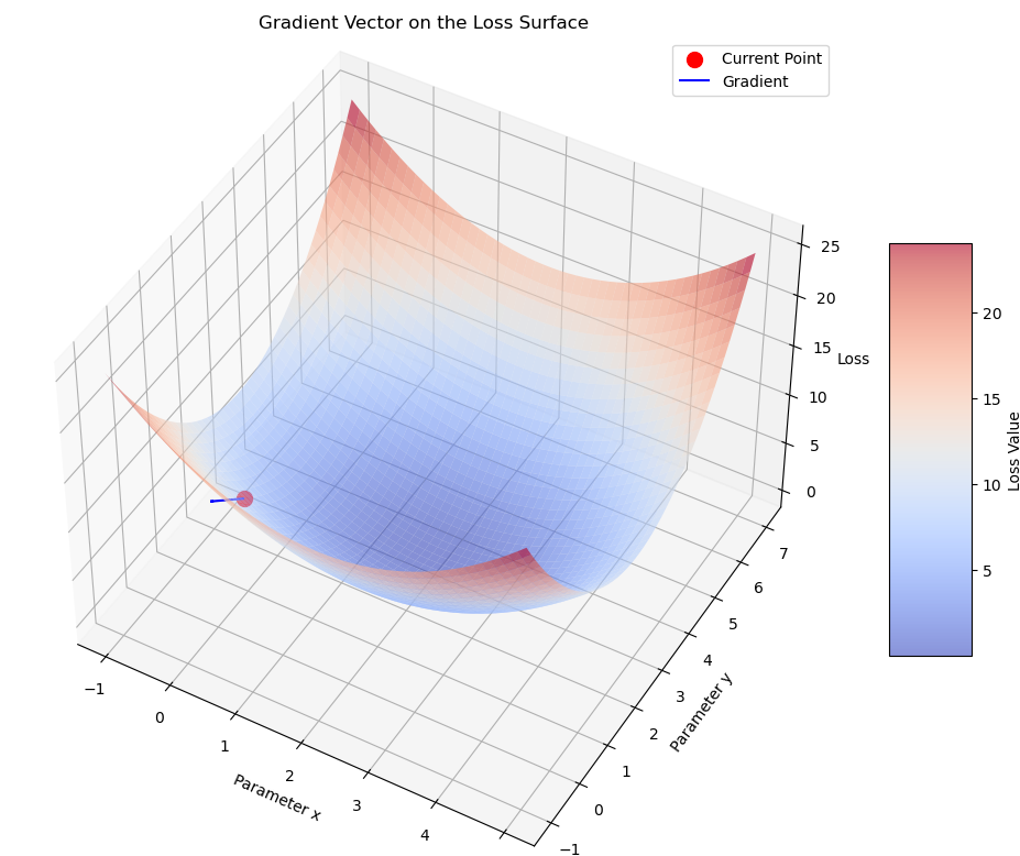
At the heart of most model training processes is gradient descent, an iterative optimisation algorithm that minimises the loss function.Here’s how it works:

• The algorithm calculates the gradient—the direction and rate of the steepest increase in loss—with respect to each model parameter.
• To reduce the loss, it takes a step in the opposite direction of that gradient.
• The learning rate determines how big that step is.

Each iteration updates the parameters slightly, gradually guiding the model toward a point where the loss is minimised.

Why gradient decent matters

Without understanding how gradients behave, you can’t diagnose training instability, vanishing gradients, or slow convergence—issues that affect every real-world ML project.

Selecting a learning rate

The learning rate controls how fast or slow the model learns.

• If the rate is too high, the model might overshoot the minimum and fail to converge.
• If it’s too low, training becomes painfully slow, or the model can get stuck in local minima.

So how do we select a learning rate?

• Start with a reasonable default (like 0.1, 0.01 or 0.001): The starting value depends on the specific model architecture and optimisation algorithm.
• Consider the magnitude of the gradients: If the gradients you observe during initial training are large, select a smaller learning rate (and vice versa).
• **Monitor the loss during training:**If the loss decreases too quickly, your learning rate is too small (and vice versa).
• Experiment and iterate. Try a few different values and observe their effect.

When to use gradient descent?

Gradient descent and its variants are used in several common model types:

Model type	What parameters are optimised
Linear regression	Finding the optimal coefficients that minimise the MSE.
Logistic regression	Learning the weights that best separate different classes.
Neural networks (deep learning)	Optimising the vast number of weights and biases in complex architectures.
Support vector machines (SVM)	Finding the optimal hyperplane that maximises margin between classes.

Let’s look at some different variations.

Batch Gradient Descent (Batch GD) This variation calculates the gradient of the loss function using theentire training dataset in each iteration. It then updates the model’s parameters based on this full gradient.How it works:

In each training step (epoch), the algorithm iterates through all the training examples, calculates the loss for each example and then computes the average gradient across all examples.

This average gradient indicates the overall direction of the steepest ascent in the loss landscape with respect to the current parameter values, considering all the training data. The parameters are then updated by taking a step in the opposite direction of this average gradient, scaled by the learning rate.

When to use it:

This variant is most suitable for smaller datasets where computing the gradient over the entire dataset is feasible.

Benefits:

• Stable convergence: Because it uses the entire dataset, the gradient estimate is accurate, leading to a more stable and often smoother convergence towards the minimum.

• Deterministic: For a given starting point and learning rate, the path to the minimum will be consistent.Risks:

• Computationally expensive for large datasets: Calculating the gradient over the entire dataset can be very slow if it is large.

• Can get stuck in local minima: If the loss landscape has many local minima, Batch GD might converge to one of them instead of the global minimum.

• Doesn’t allow for online learning: It requires the entire dataset to be available for each update, making it unsuitable for when data arrives sequentially.Stochastic Gradient Descent (SGD) Instead of using the entire dataset, this approach calculates the gradient of the loss function using only asingle, randomly chosen training example in each iteration.

The parameters are updated after processing each individual example.

How it works:

In each training step, SGD randomly selects one data point from the training set, calculates the gradient of the loss with respect to that single data point and immediately updates the model’s parameters in the opposite direction, scaled by the learning rate.

This process is repeated for the number of iterations (epochs), often shuffling the training data at the beginning of each epoch to ensure that different examples are chosen in each step.

When to use it:

SGD is more effective for larger datasets because it performs parameter updates much more frequently and with lower computational cost per update. It’s also beneficial for escaping shallow local minima due to the noisy updates.

Benefits:

• Computationally efficient for large datasets: each update is very fast since it only considers one data point.

• Can escape local minima: the noisy updates can help the algorithm jump out of shallow local minima.

• Suitable for online learning: it can process data points as they arrive and update the model incrementally.Risks:

• Noisy convergence: the gradient estimate based on a single data point can be very noisy, leading to oscillations in the loss and potentially slower convergence overall.

• Learning rate tuning is critical: the learning rate needs to be carefully tuned to ensure convergence and avoid large oscillations.

• Can be slower to reach the vicinity of the minimum: while each step is fast, the overall path to the minimum can be more erratic and might take more iterations.Mini-Batch Gradient Descent This is a compromise between Batch and Stochastic GD. It calculates the gradient of the loss function using a smallbatch of randomly selected training examples (larger than one but smaller than the total dataset) in each iteration.

The parameters are updated based on the average gradient of this batch.

How it works:

In each training step, a small subset (a mini-batch) of the training data is randomly selected. The algorithm calculates the loss and the gradient of the loss with respect to the parameters for each example in the mini-batch.

The average gradient across the mini-batch is calculated and the model’s parameters are updated in the opposite direction, scaled by the learning rate.

This process is repeated for a number of interactions (epochs), typically shuffling the data at the start of each and then iterating through the mini-batches.

When to use it:

This is the most commonly used variant in practice, especially for deep learning models. It balances the computational efficiency of SGD with the more stable convergence of Batch GD.

Benefits:

• More computationally efficient than Batch GD: processing a small batch is faster than processing the entire dataset.

• More stable convergence than SGD: averaging the gradient over a batch reduces the noise in the update.

• Can leverage vectorized operations: many computational libraries are optimized for matrix operations, which can be efficiently used with mini-batches.

• Can still escape some local minima: the noise introduced by the mini-batch sampling can help in escaping shallow local minima.Risks:

• Learning rate and batch size tuning are important: the choice of learning rate and mini-batch size can significantly affect performance.

• Convergence can still exhibit some oscillations: although less noisy than SGD, there can still be some fluctuations in the loss.

Visualising training dynamics

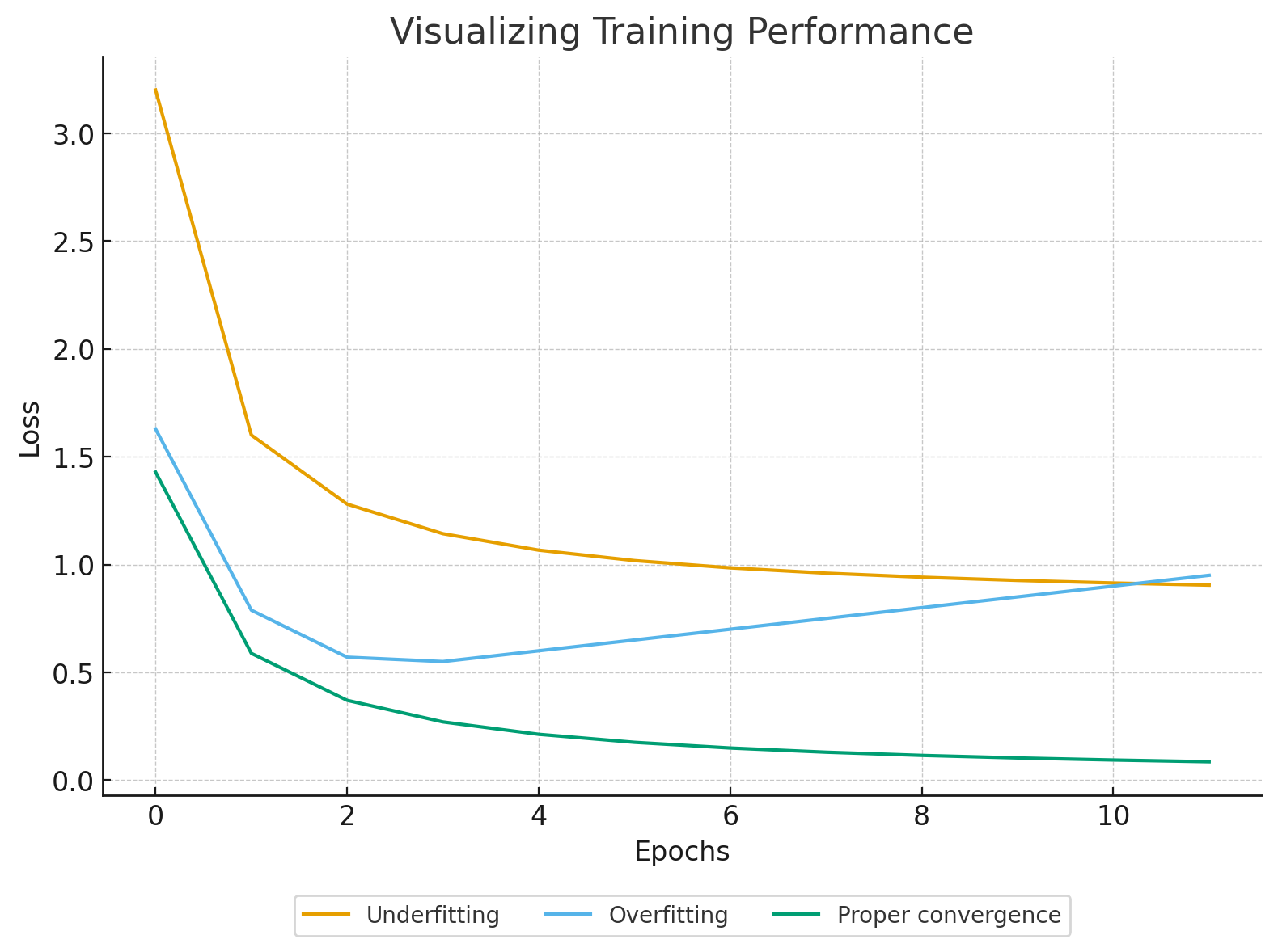
During training, we track how training loss andvalidation loss change over time. These curves tell us a lot about how well the model is learning.

Pattern	Interpretation
Both training and validation loss remain high	The model is underfitting—it has not learned enough.
Training loss drops, validation loss rises	The model is overfitting—it is memorizing instead of generalizing.
Both losses decrease and flatten together	Proper convergence—the model is well-trained and generalizes effectively.

Action item: Reflect on tuning model training

Before moving on, take a few minutes to consider the questions below.

Questions and reflections

If your training became unstable, which variable would you adjust first and why: learning rate, batch size, or number of epochs?

Your reflection here…

For your typical datasets, which gradient descent variant makes the most sense—batch, mini-batch, or stochastic—and what trade-offs come with that choice?

Your reflection here…

How would you explain the role of the learning rate to a stakeholder who only cares about delivery speed and cost?

Your reflection here…