Introduction to feature engineering

Instruction and application

In Progress

Introduction to feature engineering

So, what is feature engineering and why is it useful?

What is feature engineering?

Feature engineering is the process of transforming raw data into features that better represent the underlying problem to the predictive models, resulting in improved model accuracy on unseen data.

It involves using our knowledge of the data to create new features or modify existing ones, often by combining multiple variables, extracting meaningful components or transforming data types.

The goal is to highlight patterns and relationships in the data that might otherwise be hidden, making it easier for machine learning algorithms to learn and generalise.

Effective feature engineering is important because the quality of the features directly impacts the performance of the model, often more significantly than the choice of algorithm itself.

Why this matters

In machine learning, the quality and relevance of your input features are often the most significant factors influencing your model's performance.

Regardless of the complexity of the algorithm, models can only learn patterns that are represented in the data. If those patterns are obscured, distorted or missing due to poor feature construction, no amount of tuning will compensate.

In fact, effective feature engineering often matters more than the models we select

Simpler models generalise better: When features are clean, relevant and statistically meaningful, simpler models can capture the underlying relationships with fewer parameters and less risk of overfitting.
Interpretability increases: Good features often align more closely with domain logic, making the model's predictions easier to explain and justify.
Training time is reduced: Complex models require more computational resources. If feature engineering exposes the relevant patterns explicitly, the model doesn't need to discover them through deeper layers or ensemble logic.
Feature engineering exposes domain knowledge: Unlike automatic model tuning, the feature engineering process requires understanding the context of the data, which often yields insights useful beyond the ML pipeline.

Example: Credit default prediction

Imagine that you are building a model to predict if a customer is likely to default on their loan.

Raw features might include:

Account open date
Payment history over time (e.g. monthly balances)
Age, income, occupation

Poorly engineered features might include:

Raw strings like job titles that haven't been normalised
Dates without any transformation (e.g. account open date used as a string)
Naively averaged balance over all time, regardless of recency

Well-engineered features could include:

Number of late payments in the last 6 months
Trend in payment amounts (slope over last 3 months)
Days since account opening
Normalised debt-to-income ratio
Binary flag for high-risk employment types

Creating these new features using the available information may help boost the performance of the model.

Overview of the feature engineering workflow

Feature engineering is not a one-step process. It is a workflow composed of several stages. Each informs the next and depends on the choices made before it.

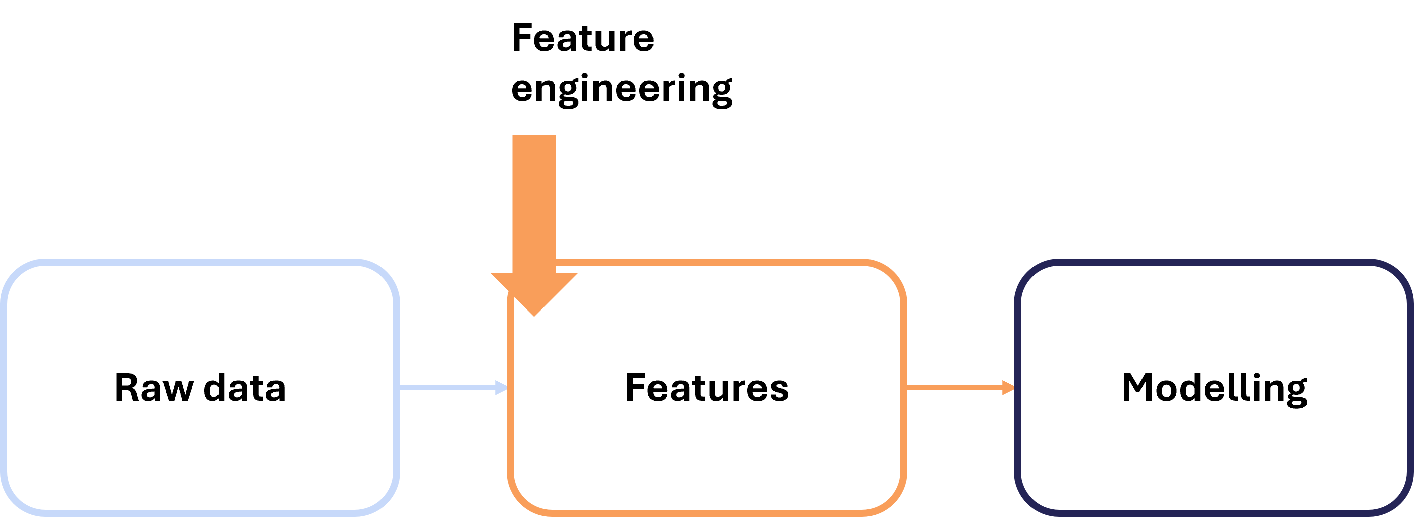
The overall goal is to extract powerful predictive features from raw data in a way that reflects domain realities, supports the assumptions of your learning algorithm and improves model generalisation.

Let's take a look at what a typical flow might look like.

1. Understanding the domain and data sources

You could create sophisticated features that extract meaningful information from raw data, but if you don't understand its context, you are more likely to create useless features that might make the model worse.

The first step in feature engineering is understanding the context of your data and where it comes from.

Why it matters

ML models don't know what the data means. They only know how it behaves mathematically. That is why it is important that you begin by understanding the source, purpose and structure of the data.

Without this context, you risk building features that are misaligned with the problem, introducing subtle forms of leakage or encoding unintended bias.

Steps:

Clarify the unit of analysis: Is each row a customer, a transaction or a sensor reading? This affects how you aggregate and interpret patterns.
Identify event types and timeframes: What kind of events are logged, and what temporal scope does the dataset cover? This impacts which temporal features you can construct (e.g. lagging metrics, rolling windows).
Interview stakeholders or SMEs: Talk to product managers, analysts, engineers or domain experts to clarify field definitions, data collection quirks or edge cases.
Trace the data lineage: Understand how each column was created. Was it calculated upstream, entered manually or derived from another source? This helps identify proxy features or leakage risks.

Red flags to catch early

Variables that seem predictive but leak future information (e.g. labels encoded into training data).
Ambiguous categorical fields with overloaded meaning (e.g. 'status' could mean account status, legal standing or eligibility).
Features with unstable definitions over time or between populations (e.g. location coded differently in different regions).

2. Exploratory data analysis

Once you have understood your data, the next step is to explore it to find out what relationships and behaviours it contains.

This will help you identify what is possible and start planning what new features you might be able to engineer.

Why it matters

You cannot engineer meaningful features without first understanding how your existing features behave.

Data exploration surfaces the hidden assumptions, irregularities and non-linearities that can later be addressed through transformations or new feature design. This phase helps translate domain concepts into statistical patterns.

Steps:

Plot the data: Visualise distributions of individual variables using histograms, boxplots and density plots. Look for skewness, heavy tails, spikes at zero and similar patterns.
Missing data analysis: Quantify missing data per column, explore co-occurrence patterns in missing values and determine whether missing data is systematic.
Outlier detection: Use interquartile ranges or z-scores to detect extreme values. Determine whether these outliers are errors, rare cases or meaningful deviations.
Group-wise analysis: Aggregate by cohort (e.g. user segment, time window, geography) to spot structured heterogeneity.

Insights to capture

Which variables are correlated with the target, and are those correlations stable across groups?
Where might a log transform normalise variance?
Are there obvious interaction effects (e.g. age and income together predict churn better than either alone)?
Have patterns drifted over time (e.g. seasonality or behavioural shifts)?

3. Creating new features from raw data

Once you have understood your data and its patterns, you are in a position to start engineering new features.

Let's take a quick view of what types of transformations you might want to use.

Mathematical transformations

Sometimes a new feature can be created from applying a mathematical technique to rescale a feature or transform its distribution.

Let's review common transformations:

Log-scaling

This compresses large values while expanding smaller ones, making the variable more normally distributed. For example, if a monetary feature ranges from $10 to $100,000, a log-transform will reduce the dominance of larger values in the model.

When to use it: When your data is heavily right-skewed (e.g. income, number of daily logins).

Square or cube root

Similar to log-scaling, but softer, reducing skew and variance without completely squashing differences at the high end.

When to use it: Useful for count data (e.g. number of purchases or clicks).

Polynomial transformations

This captures non-linear effects in a linear model. For example, churn may be high for both very low and very high engagement levels.

When to use it: When the relationship between the feature and target is non-linear (e.g. U-shaped or exponential).

Temporal features

If our data is time-based, we can extract behavioural patterns, recency effects, decay and seasonality, which can be influential in a model.

Examples:

Days since last event: Captures how long it has been since an important event has happened (e.g. age of account, days since last payment or appointment).
Rolling metrics over fixed windows: A descriptive statistic that travels through a time series, recalculating over new and consecutive windows (e.g. showing how average usage of a product has changed over time).
Change over time (slopes or deltas): Tracks how the data has been trending over time, for example, if more or less customers are using a product each day.

Aggregation features

Instead of using the raw data, we can compress it by aggregating it on a categorical feature and calculate a summary statistic to represent it.

Types of aggregations:

Counts: Total number of events, interactions or sessions.
Means and medians: Useful for smoothing out high-variance behaviour.
Standard deviation or variance: Measures behavioural volatility.
Max/min: Often used to flag extreme behaviours.
Quantiles (25th, 75th, etc.): Provide more robust insight than means when data is skewed.

Interaction features

These model the relationship between variables, often non-linearly, to expose dependent behaviour not visible in exploratory data analysis.

Examples:

Multiplicative interactions: Capture proportional or compounded effects. For example, calculating clicks x ad_cost can indicate campaign efficiency.
Ratios and rates between features: Encode relative usage or imbalance. For example, cart_items / visits can signal purchase intent, and spend / number_of_items reflects average cart value.
Deltas or change over time: Measure the difference between values across time steps. For example, daily change in account balance or slope in payment behaviour over a recent window.
Boolean or categorical combinations: Create new levels or groups based on conditions which are evaluated as true or false. For example, you could create a field that is true or false if someone is high income and rural.

Missing value flags

One often overlooked but powerful feature engineering strategy is to create Boolean flags indicating whether a value was missing in the original dataset.

For example, a new feature like income_missing = True can be highly predictive, especially in domains like credit risk or churn modelling, where the absence of data may reflect user intent, disengagement or systemic bias.

These indicators help surface patterns that traditional imputation or deletion might obscure, and are often especially valuable in real-world, messy datasets.

Domain-specific metrics

This is a catch-all category for any metric that is specific to the domain you are working in and can be useful as a predictive feature.

Examples:

Finance: debt-to-income ratio.
Marketing / SaaS: net promoter score.
Health care: body mass index.
E-commerce / Retail: conversion rate.
Operations / Logistics: average fulfilment lag.

4. Selecting the most useful features

So you have engineered some new features for your model, but will they be useful?

The more features you input, the more complex the model becomes, which can result in overfitting. It is important that we check that these new features are going to improve our models and not make them biased or more complicated than necessary.

Why it matters

Feature selection improves model performance, speeds up training and simplifies interpretation. Including every possible feature, especially correlated or irrelevant ones, can lead to multicollinearity, noise amplification or overfitting.

Techniques and strategies

Filter methods: Use correlation thresholds, mutual information scores or chi-square tests to remove uninformative or redundant features before modelling.
Wrapper methods: Recursive Feature Elimination (RFE) or sequential feature selection evaluate feature subsets based on model performance.
Embedded methods: Let the model determine feature importance internally (e.g. LASSO for linear models, Gini importance for trees).

Evaluation techniques

Cross-validation: Estimate model performance on unseen data. Compare feature sets across folds.
Feature ablation tests: Drop one feature or group at a time to measure performance impact.
A/B testing of feature sets: Compare models with and without engineered features under the same training regime.
Model diagnostics: Examine residuals, confusion matrices, ROC curves or SHAP values to see where features help.

Working through this workflow, you will be able to identify new features that might improve the performance of your models.

More sophisticated models can reduce interpretability, so engineering new features may allow simpler models to work more effectively.

If you are developing a model, consider what features you might want to engineer and see if they can improve performance while also not adding too much complexity.

Different use cases

In this section, we have looked at several feature engineering strategies. To help you recognise when to use each, we have summarised the different use cases in this table.

Strategy	Core goal	Typical use cases
Improvement	Clean and normalise raw features	Any numeric modelling
Construction	Inject domain logic and pattern recognition	Time series, business intelligence
Selection	Reduce noise and overfitting	High-dimensional tabular data
Extraction	Collapse redundant features	Sensors, text, images
Learning	Discover abstract structure automatically	Deep learning, unstructured data

Feature engineering tools: Python open source libraries

What Python libraries are available for feature engineering?

This table summarises some of the more common ones you might encounter.

Tool	What it is
Featuretools	Automatically generates meaningful features from relational and time-indexed data.
Scikit-learn	The most widely used machine learning library in Python, with extensive modules for feature selection, preprocessing, model training and pipeline automation.
Feature-engine	A powerful alternative and complement to Scikit-learn's preprocessing tools, designed specifically for interpretable, human-centred feature engineering in tabular datasets.
TSFRESH	A specialised Python package that automatically extracts hundreds of statistical features from time-series data, including Fourier coefficients, entropy, autocorrelations, peak detection and more.
NLTK	The go-to library for foundational NLP tasks in Python: text tokenisation, lemmatisation, part-of-speech tagging and feature vector construction from raw text.
Category Encoders	A robust collection of categorical encoding schemes that go beyond one-hot and label encoding, enabling more effective handling of high-cardinality and informative categorical data.
Boruta	A wrapper method designed not just to find a minimal subset of features but to identify all features that have a statistically significant association with the target. It is particularly well suited to scenarios where weak but meaningful predictors exist, such as biological, financial or behavioural modelling contexts.

Tip

These libraries, when used together, offer a full-stack solution for feature engineering across many data types.

Learning when and how to use them will improve your ability to build smarter features, reduce noise and construct models that generalise well.

Action item: Introduction to feature engineering checkpoint

Let's see if you can apply what you've learnt by answering the questions in the next activity.