Validating model improvements with statistical tests
 Instruction and application
 In Progress
Validating model improvements with statistical tests
You've calibrated your model and improved its confidence scores—but how can you tell if these improvements really matter?Not every improvement in model performance is meaningful—random fluctuations or data splits can easily mislead. In this section, you’ll learn how to design fair comparisons and apply statistical tests that distinguish real gains from lucky noise.
You’ll explore four common tests—each suited to different model outputs and use cases—and see how they help guide confident, evidence-based refinement decisions.

Setting up experiments to compare model variants
Before you apply any statistical test, your comparison setup must be sound. Poor experimental design can create misleading results—even if your math is flawless.
Select the tabs to learn how to make your experiment setup fair and reproducible:
** Use identical data splits across all models** This ensures you’re comparing model behavior on the same examples. Changing the test set can introduce variation unrelated to model quality.** Align evaluation metrics and thresholds** If one model is scored on precision at 0.5 and another at 0.7, you’re not making a like-for-like comparison. Keep your metrics and thresholds consistent.** Repeat with cross-validation or multiple runs** A single train/test split can misrepresent real performance. Use k-fold cross-validation or repeat experiments with different seeds to reduce randomness.** Control for confounding variables** Especially if you're comparing models trained on different hardware or time periods—log everything, and isolate your variable of interest (the model itself).
These practices lay the foundation for statistical tests to be ** trustworthy** and** actionable**—not just technically correct.
Statistical tests for performance differences
Here are four common tests used in ML model evaluation. Each helps answer a different version of the question: Is the performance difference I see actually real?** T-Test: Comparing mean scores**
The paired t-test checks if two models have significantly different performance scores (e.g., accuracy or F1) over repeated runs or folds.** Use when:**
- You're comparing numeric scores from the same data folds.
- The performance differences are roughly normally distributed.** Formula:** t = (mean₁ − mean₂) / (std_diff / √n)
T-Test - Worked example
You run 10-fold cross-validation for two logistic regression models—one with L2 regularisation, one without. Their F1-scores on each fold are:** Solution**
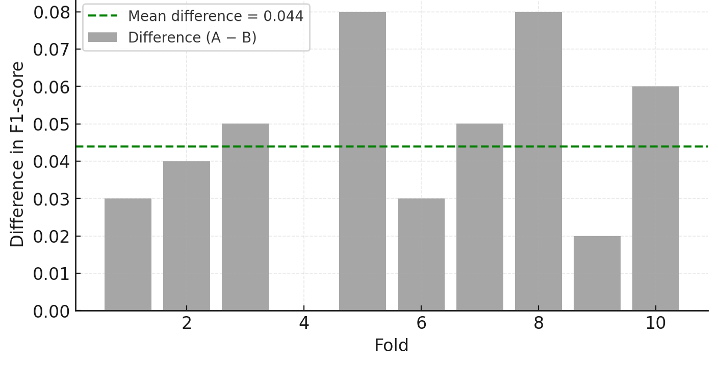
- ** Step 1:** Compute fold-level differences (A − B): [0.03, 0.04, 0.05, 0.00, 0.08, 0.03, 0.05, 0.08, 0.02, 0.06]
- ** Step 2:** Mean difference = 0.044
- ** Step 3:** Standard deviation of differences ≈ 0.025
- ** Step 4:** Apply the formula:** t = 0.044 / (0.025 / √10) ≈ 5.56** As shown in the diagram below, the gray bars represent the fold-level differences in F1-scores between the two models. The green dashed line shows the mean difference across all folds, which is what the t-test uses to determine if the improvement is statistically significant.
In this case, the t-value of 5.56 indicates that the improvement from adding L2 regularisation is very unlikely to be due to random variation. The difference is statistically significant, suggesting the regularised model generalises better across folds.
Cohen’s Kappa: Measuring agreement beyond chance
Cohen’s Kappa measures agreement between two classification models, correcting for what could occur by chance.** Use when:**
- You're comparing label predictions, not probabilities.
- You want to assess consistency between models.** Formula:**
κappa = (pₒ − pₑ) / (1 − pₑ)
Where:
- pₒ = observed agreement
- pₑ = expected agreement by chance
What do we mean by agreement?
- Observed agreement (pₒ): The percentage of times both models made the same prediction.
- Chance agreement (pₑ): The percentage of agreement you'd expect just by chance—based on the distribution of predicted classes. Kappa = (pₒ − pₑ) / (1 − pₑ) adjusts for this and reveals whether models truly align in their decisions.
Cohen’s Kappa - Worked example
Two models are classifying 1,000 emails as spam or not spam.
-
They agree on 820 emails.
-
Due to class imbalance (most emails are not spam), the expected chance agreement is 65% (pₑ = 0.65).** Solution**
-
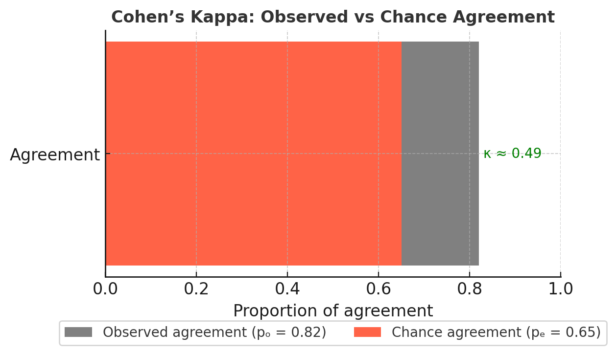
** Step 1:** Observed agreement (pₒ): pₒ = 820 ÷ 1000 = 0.82
-
** Step 2:** Apply the formula: κ = (0.82 − 0.65) ÷ (1 − 0.65) κ = 0.17 ÷ 0.35 κ ≈ 0.49 As shown in the diagram below, the gray portion represents the observed agreement (82%), while the red portion represents the part of that agreement that could be explained by chance (65%). Cohen’s Kappa isolates the difference, showing how much agreement remains once chance is removed.
A κ value of about 0.49 indicates ** moderate agreement** between the two models. Even though raw agreement was 82%, nearly two-thirds of that could have been due to chance. Kappa corrects for this, giving a truer sense of model alignment.
McNemar’s Test: Spotting label shifts
McNemar’s Test is used to compare the error patterns of two binary classifiers on the ** same dataset** . It focuses on cases where the models** disagree** , helping you detect if one consistently makes better decisions—or if performance differences are just noise.** Use when:**
You’re comparing two models that output yes/no or positive/negative predictions. You want to know if their errors differ in a statistically meaningful way.** How it works:**
McNemar’s Test uses a ** 2×2 disagreement matrix**:** Model B: Correct** ** Model B: Wrong**** Model A: Correct** a (agree)b (disagree)** Model A: Wrong** c (disagree)d (agree)
The test focuses only on ** b and c**—the cases where the models** disagree** .
If b ≠ c, there may be a real difference in performance.** Formula:**
χ² = (|b − c| − 1)² / (b + c) Example: Fraud detection model comparison You’re evaluating a new fraud detection model against an existing one. Both models are tested on the same transactions.
- They agree on most cases—but disagree on a small subset.
- Model A flags 30 transactions that Model B misses.
- Model B flags 10 that Model A misses. McNemar’s test uses these asymmetries (30 vs. 10) to calculate whether the difference is likely meaningful—or just noise due to data variation.
The following matrix captures this disagreement, and the result tells you if it’s worth switching to the new model.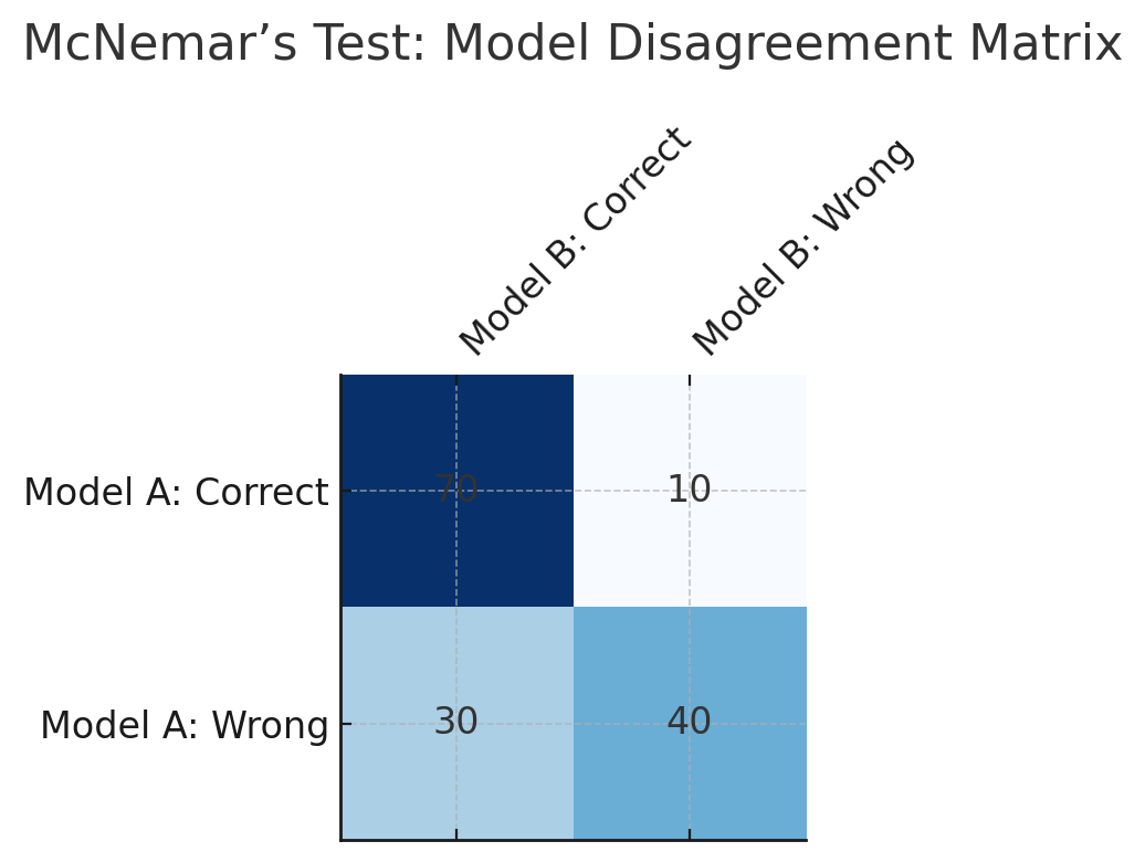
** Applying the formula to our example:** You observed:
-
b = 30 cases where Model A was correct but Model B was wrong.
-
c = 10 cases where Model B was correct but Model A was wrong. Plug these into the formula:
-
χ² = (|30 − 10| − 1)² / (30 + 10)
-
χ² = (19)² / 40
-
χ² = 361 / 40
-
χ² ≈ 9.03 Depending on your chosen significance level (e.g., p < 0.05), a χ² value this high would indicate that the difference is statistically significant.** Interpretation:** The new model is making meaningfully different decisions—not just random changes. That supports your case for deploying it, especially if those differences align with your business goals (e.g., catching more fraud).
Permutation Test: When you can’t assume normality
Sometimes your data won’t fit the nice bell curve needed for other tests. That’s where the permutation test comes in—a flexible, non-parametric approach that doesn’t rely on normal distribution assumptions.
Instead of fitting equations, this method simulates random chance by shuffling predictions and recalculating the result many times. If your observed improvement happens more often than not in these shuffles, it’s probably not significant.** When to use it:**
- Your metric (e.g. AUC, log loss) is not normally distributed.
- You want a distribution-free way to test whether performance differences are real.
- ** You’re comparing models on the same dataset or under the same conditions.**
** How it works:**
- Calculate the actual performance difference between the two models (e.g., Model A AUC − Model B AUC).
- Shuffle the model predictions or labels randomly between the two models thousands of times.
- Record the new differences after each shuffle.
- Compare: How many shuffled differences are greater than or equal to the original? That’s your p-value.** Example: AUC comparison in deep learning**
You’ve trained a new deep learning model that slightly outperforms your baseline—AUC improves from 0.82 to 0.845. To test if this gain is real, you apply a permutation test:
- You ** shuffle** predictions between models 1,000 times.
- ** Only 9** of those shuffles produce a greater AUC difference than your original 0.025.** Result:** p-value = 9 / 1000 = 0.009 → The improvement is ** statistically significant** .
In the following histogram, the red line shows your model’s observed performance gain. The bars show how often random shuffles produced each difference. Since very few fall beyond your result, you can be confident your model’s improvement is real—not random.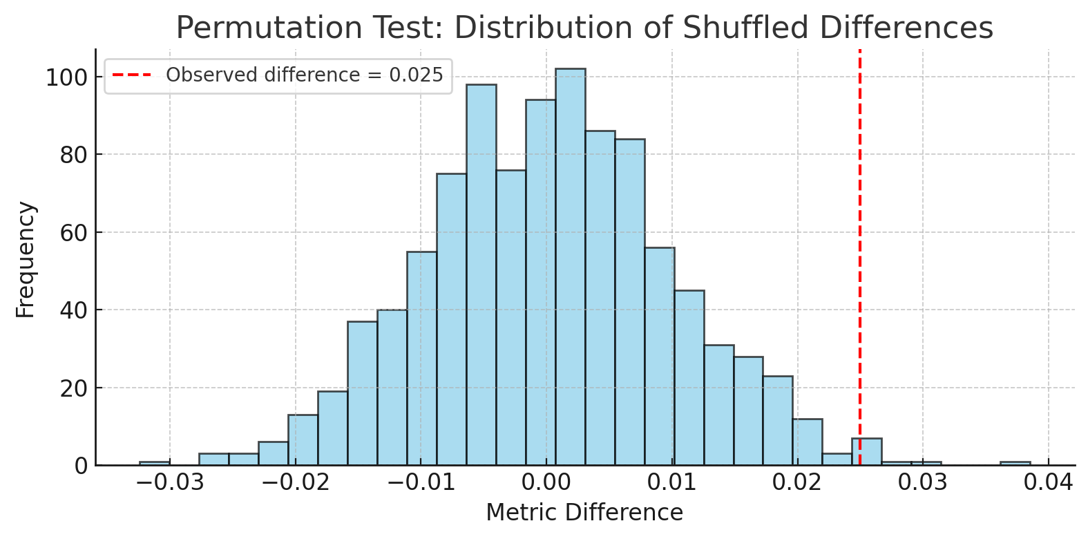
** Case study: How evaluation insights drive model refinement**
A national retail company is trying to reduce customer churn. Their data science team has trained two high-performing models:
- A ** gradient-boosted tree** model.
- A ** calibrated neural network** with probability output adjustment. Both models achieve similar AUC scores on the held-out test set—so at first glance, they seem equally effective. But the business wants to know: which model is actually better for catching real churners and guiding targeted retention efforts?
Test for average performance difference
They begin with a ** paired t-test** to compare AUC across 10-fold cross-validation runs.** Result**: No statistically significant difference.** Conclusion**: Average scores aren’t enough to distinguish the models.
Examine prediction differences
Next, they run ** McNemar’s Test** to compare the two models’ predictions on the same dataset. This test reveals:
- The neural net ** correctly identifies more actual churners** .
- It ** doesn’t increase false positives** compared to the tree model. This shift isn’t just noise—McNemar’s Test confirms it’s statistically significant.
Business decision
The team presents both results to leadership:
- The ** t-test** says average AUC is a tie.
- The ** error pattern analysis**(via McNemar’s Test) shows the neural net catches more customers who actually churn—without wasting resources on false alarms.
Final decision
The company deploys the ** neural net** model—not because it scored higher, but because its improvement translates to real business value: saving more customers.
Action item: Reflect and apply
Think about model comparisons you’ve made—or ones you might make soon.
Take a moment to capture your reflections using the form below. Thinking through these questions now will make it easier to apply the right techniques when the stakes are high.