Optimising for sustainability and efficiency

Instruction and application

Complete

Optimization techniques for model training

So far, we have looked at how we can measure the performance of our models, but what can we do to improve them?

In this section, we are going to explore some optimization techniques that can help us overcome common challenges when training our models and achieve better results.

Regularization methods

A common issue we come across when training models is overfitting. This is when the model adapts too well to the noise and patterns found in the training data and cannot generalize to new data, making the model useless for deployment.

Regularization techniques help prevent overfitting by adding a penalty to the model’s loss function, discouraging overly complex models.

Let’s take a look at some common techniques.

**L1 Regularization (Lasso regression)**If you have a dataset with high-dimensionality (i.e. a large number of features), a model will struggle to find the relationships in the data without overfitting.

Lasso regression penalizes the absolute size of the coefficients, driving some to zero. This effectively results in a form of feature selection, resulting in a more sparse and interpretable model which focuses more on the features with more influential coefficients.

How it works:

L1 regularization adds the absolute value of the magnitude of the coefficients as a penalty term to the loss function.

Mathematically, we represent the loss function as where the parameters are represented by , The L1 regularized loss function is:

Where is the regularization strength (a hyperparameter) and is the number of features.

This penalty encourages the coefficients of less important features to become exactly zero, effectively performing a feature selection.

Choosing an appropriate regularization strength ():

• Cross-validation: The most reliable method is to use k-fold cross-validation. Train and evaluate your model with different values of on the validation sets and choose the that yields the best performance (e.g. lowest validation error).

• Information criteria: Techniques like AIC (Akaike Information Criterion) or BIC (Bayesian Information Criterion) can provide guidance, balancing model fit and complexity.

• Grid search or randomized search: Systematically search through a range of values. Logarithmic scales are often useful for exploring a wide range effectively.When to use:

• **When feature selection is desired:**If you suspect that many features are irrelevant and want to automatically select the most important ones, this leads to simpler and more interpretable models.

• **Sparse solutions:**If you want a model with only a few non-zero coefficients.

• **High-dimensional datasets:**If your data has more features than number of samples.**Benefits: **

• Automatic feature selection: If you have many features and are not sure which ones will be useful, this technique will simplify your model and improve interpretability.

• Robust to irrelevant features: If you include features which turn out to be useless and cause noise, lasso regression will remove them.Risks:

• Can be too aggressive: The penalty is applied indiscriminately and can result in slightly useful features being removed, potentially causing underfitting if is too large.

• Non-differentiable at zero: The absolute value function is not differentiable at zero, which can sometimes complicate complex algorithms, although modern solvers handle this well.L2 Regularization (Ridge Regression)

Unlike lasso regression which penalizes unimportant features, ridge regression looks to reduce the impact of large coefficients by penalizing the squared size of the coefficients, shrinking them all towards zero.

We use ridge regression when all features are potentially relevant, aiming to improve generalization and reduce multicollinearity.

How it works

L2 regularization adds the squared magnitude of the coefficients as a penalty term to the loss function . The L2 regularized loss function is:

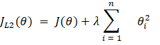
Where is the regularization strength (a hyperparameter) and is the number of features.

This penalty discourages large coefficient values, effectively shrinking them towards zero but rarely making them exactly zero. This helps to reduce the impact of highly influential individual features.

Choosing an appropriate regularization strength ():

• Cross-validation: just like with L1, k-fold cross-validation is the standard approach to find the optimal λ that minimizes validation error.

• Generalized cross-validation (GCV): an efficient way to estimate the prediction error for different values of λ without explicitly splitting the data into folds.

• Regularization path algorithms: algorithms like LARS (Least Angle Regression) can efficiently compute the coefficient paths for a range of λ values, aiding in selection.When to use:

• All features are potentially useful: When you believe that most features contribute to the outcome to some extent.

• Reducing multicollinearity: If you have highly correlated features, ridge regression shrinks their coefficients, which can help stabilize the model.Benefits:

• Computationally easier: The squared term makes the loss function differentiable everywhere, which allows the model to work more efficiently.Risks:

• No feature selection: All features are retained with this method (although their influence is reduced), so irrelevant features can still have an impact.

• Less interpretable than L1: As it retains all features, it can be more difficult to interpret the model in terms of identifying the key players behind predictions or inferences.Elastic Net Regularization

Why choose between L1 and L2 regularization when you can have both?

That’s what Elastic Net does, it combines the L1 and L2 penalties to get the benefits of both feature selection and handling correlated features. If you are working with high-dimensional data that has multicollinearity, this method will help obtain a balance between sparsity and stability.

How it works

Elastic Net is a hybrid approach that combines both L1 and L2 regularization. It adds a penalty term that is a linear combination of both:

Where is the regularization penalty of lasso regression (L1) and is the regularization penalty from ridge regression (L2).

Often, the formula is parameterized with a single regularization strength and a mixing parameter , where :

If you set = 1 you get lasso regression and = 0 gives you ridge regression.

Choosing the appropriate regularization strengths ( and ):

Nested cross-validation: due to the presence of two hyperparameters, nested cross-validation is the recommended approach (i.e. run one “outer” loop to evaluate the model’s performance and “inner” loops to find the optimal hyperparameters).

• The “outer loop” estimates the generalization performance and hyperparameter tuning process. It splits the data into several “outer folds”.

• For each outer fold in the iteration:The remaining outer folds are used as training data for an inner cross-validation loop. This inner loop is responsible for finding the best and for the model.

• It splits the inner training data into several inner folds.

• For each combination of hyperparameters it trains the model on a subset of the inner training folds and evaluates it with the rest.

• The hyperparameters that give the best performance in the inner loop are then used to train a model on the entire outer training set.

• This trained model is then evaluated on the held-back outer test fold. Grid search or randomized search (2D): we can explore combinations of and and see which returns the optimal performance.When to use:

• High-dimensionaland correlated data: Elastic Net is what you should choose if you have both problems of too many predictive features and multicollinearity. The L1 regularization will remove irrelevant features, while the L2 regularization will shrink the coefficients, providing a balanced approach.Benefits:

• Combines L1 and L2 regularization: we can perform feature selection and handle multicollinearity effectively.

• More flexible: the mixing parameter allows us to tailor the regularization to the specific characteristics of our data.Risks:

• More complex hyperparameter tuning: as this approach requires two hyperparameters to be optimized, the process can be more computationally expensive.Dropout

The previous regularization methods are used most commonly with regression models, but what about other model families?

Dropout is a technique used when training deep neural networks, particularly in fully connected layers, to prevent overfitting.

It works by randomly deactivating neurons during training to prevent over-reliance on specific neurons and improve generalization.

How it works

During training, dropout randomly selects a subset of neurons (and their connections) to be temporarily “dropped out” with a certain probability . This means these neurons do not contribute to the forward or backward pass for that particular training iteration.

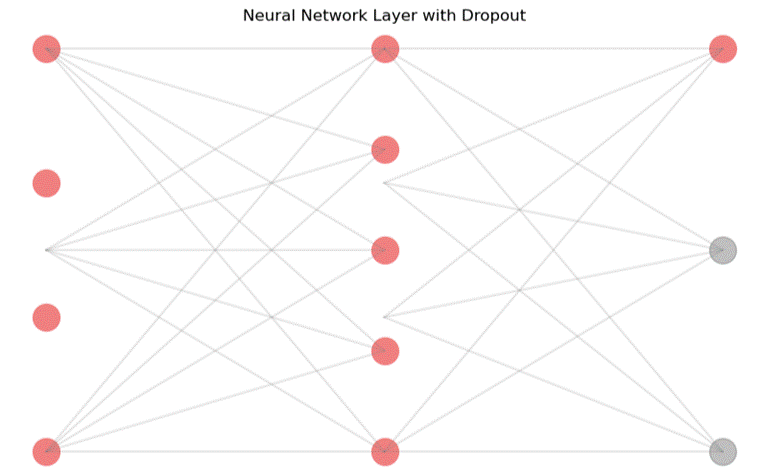
The process forces the network to learn redundant representations, as no single neuron can rely on the consistent presence of its neighbors. It effectively trains an ensemble of thinned networks.

During inference, all neurons are active, but their weights are typically scaled down by the dropout probability to account for the fact that more neurons were active during training.

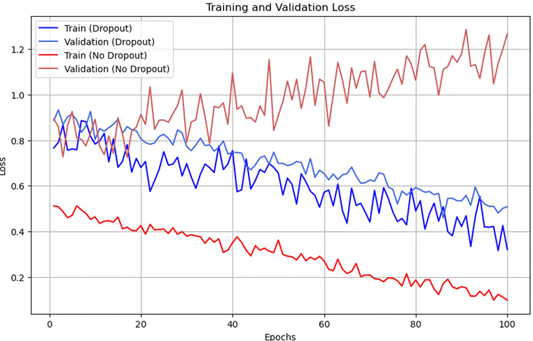
Choosing the appropriate dropout rate ():

• Common values: dropout rates are usually chosen between 0.2 and 0.5. Lower rates (i.e. 0.1 or 0.2) have a smaller regularization effect, while higher rates (0.5) can lead to significant underfitting if not used carefully.

• Layer-specific tuning: the optimal dropout rate can vary between layers of the network. It is common to apply higher dropout rates to the fully connected layers, which tend to have a large number of parameters and are more prone to overfitting.

• Cross-validation: experiment with different dropout rates using cross-validation on your validation set to find the rate that yields the best performance.When to use:

• Deep neural networks: dropout is particularly effective when the neural network has many parameters.

• Fully connected layers: often applied to the fully connected layers of a convolutional neural network (CNN) or recurrent neural network (RNN).Benefits:

• Reduces co-adapation of neurons: makes the network more robust and less reliant on specific combinations of features.

• Implicit ensemble learning: can be seen as training and averaging the predictions of many thinned networks.Risks:

• Underfitting: too high a dropout rate can lead to significant information loss and underfitting, where the model fails to learn the underlying patterns in the data.

• Increased training time: dropout can slow down the training process as the network has to learn multiple sub-networks.Other regularization techniques for neural networks:

• Weight decay (L2 regularization): Apply L2 regularization directly to the weights of the neural network layers, penalizing large weights.

• Batch normalization: Normalize the activations of intermediate layers, stabilizing training and providing a subtle regularization effect.

• Early stopping: Monitor validation performance and stop training when it starts to degrade.

• Data augmentation: Create modified versions of the training data to increase its diversity and force the model to learn more generalizable features.

• L1 weight regularization: Apply L1 regularization to the weights, encouraging sparsity in the weight matrices.

• Activity regularization: Penalize the activation of neurons, encouraging sparsity (L1) or smaller values (L2). Regularization techniques are effective for addressing overfitting in our models. If you are using large data which risks multicollinearity or a large number of features, try using some of these techniques and see if it improves your model’s performance.

Key points

To improve model performance and overcome challenges like overfitting, we can apply several optimization techniques.

• Regularization methods such as L1 (Lasso), L2 (Ridge), and Elastic Net help control model complexity and improve generalization by penalizing large or unnecessary coefficients.
• In deep learning, techniques like Dropout prevent over-reliance on specific neurons, promoting more robust models.
• Additional strategies—including early stopping, batch normalization, and data augmentation—further enhance model performance and reduce overfitting. By carefully selecting and tuning these techniques, we can develop models that not only perform well on training data but also generalize effectively to unseen data.

Action item: Pause and think.

Before moving on, take a few minutes to consider the questions below.

Hyperparameter tuning

What if a few small tweaks could dramatically boost your model’s performance?

Hyperparameters are like hidden dials that control how a ML model learns. Tuning them correctly can be the difference between a model that barely works and one that delivers game-changing insights.

In this section, you’ll learn how to systematically fine-tune these critical settings to improve accuracy, reduce errors, and unlock your model’s full potential.

Regularization methods

Hyperparameters are the “knobs and dials” of a ML model. They dictate aspects of the training process and the model’s architecture, influencing how the model learns and ultimately performs.

Examples include the learning rate in gradient descent, the number of layers in a deep neural network or the regularization parameter in a ridge or lasso regression.

Poorly chosen hyperparameters can lead to:

• Underfitting: Where the model fails to capture the underlying patterns in the data.
• Overfitting: Where the model picks up too much of the noise in the training data and does not generalize well to new data.
• Suboptimal performance: Where the model does not achieve its full potential (even if it avoids over or under fitting). This is why hyperparameter tuning is important. It is the process of systematically searching for the optimal combination of these settings to achieve the best possible model performance on unseen data.

Let’s explore some common techniques.

Grid searchImagine you have several hyperparameter settings to test, what would be the most simple way to find out which combination is the most effective?

You try all the combinations!

This is how Grid Search works, it is an exhaustive method which evaluates each possible combination of hyperparameters by training and evaluating a model for each.

How it works: Imagine that you are training a neural network with two hyperparameters- learning rate and number of hidden units, selecting following values to test:

• Learning rate - 0.01, 0.001 and 0.0001.
• Hidden unit counts - 32, 64 and 128. Grid search trains and evaluates a model for every possible pairing (e.g. 0.01 & 32, 0.001 & 32, etc). The combination that yields the best performance is selected.

When to use it:

Grid Search is most effective when you have a relatively small number of hyperparameters to tune and a limited range of potentially good values for each.

It’s also a good starting point when you have some intuition about the likely ranges of optimal hyperparameters.

Benefits:

• Guaranteed exploration: As the algorithm systematically explores all defined combinations, it ensures that you do not miss out on potentially good settings.

• Easy to understand and implement: The concept is quite straightforward - you try every possible combination to see which works best.Risks:

• Computationally expensive: The number of combinations grows exponentially with the number of hyperparameters and the size of their value sets. If you have a lot of hyperparameters, this approach will not be efficient.

• Inefficient for continuous or very wide ranges: To use Grid Search, you define a discrete number of values to test. If the optimal value is between two of them, you will miss it.**Random search **While Grid Search tries every possible combination of hyperparameter values, Random Search picks a random value from a defined distribution for each.

To use it, we specify a range or probability distribution (e.g. uniform, normal) for each hyperparameter and then set a “budget” for a number of trials (the number of combinations we want to evaluate).

How it works

Instead of trying every combination, we pick a random value for each hyperparameter from its specified distribution for a fixed number of iterations.

Going back to our previous example of a neural network with two hyperparameters, we might specify the following:

• For the learning rate, a logarithmic uniform distribution between 0.0001 and 0.1.
• For the hidden units, a uniform distribution between 32 and 128.

The algorithm then randomly samples a learning rate and a number of hidden units for each trial, trains a model and evaluates its performance.

How to select a distribution:

Selecting an appropriate distribution for your hyperparameter is important. If you have good prior knowledge or intuition, then you should be able to select one which is appropriate.

Otherwise, start broad with a wider distribution and refine.

This table summarizes some distributions for different types of hyperparameter.

Continuous, unbounded or very wide ranges- Uniform

• Logarithmic uniform (useful if the optimal values span several orders of magnitude) Continuous, with a known or suspected reasonable range- Uniform
• Normal (if you have likely good value from some prior belief) Integer values with a reasonable range- Discrete uniform Categorical hyperparameters- Discrete uniform (over the possible categories) When to use it:

If you have hyperparameters that are significantly more important than others, this technique will often outperform Grid Search. It is also more likely to find good values for important hyperparameters within a given computational budget as it is not looping through discrete values. It’s also useful when you have less intuition about the optimal ranges and want to explore a wider set of values.

Benefits:

• More efficient than Grid Search for high-dimensional data: By random sampling, it is more likely to stumble upon good combinations, especially when some hyperparameters have a limited impact.

• Can explore a wider range of values: You can define continuous ranges or probability distributions, allowing for more granular exploration.Risks:

• No guarantee of exploring all defined values: Unlike Grid Search, some possible values for your hyperparameters might be missed entirely.

• Performance can be sensitive to the number of trials: A very small number of trials might not be enough to find good values for your hyperparameters.Bayesian optimizationThis is a more intelligent and efficient approach to hyperparameter tuning. Bayesian optimization uses a probabilistic model to reason about which hyperparameters are likely to yield the best performance.

It iteratively builds a surrogate model (typically using a Gaussian Process) of the objective function (the performance metric we want to optimize) and uses this model to decide which hyperparameter configuration to evaluate next.

How it works:

Bayesian optimization follows this process:

• Initialization: It starts by evaluating a few randomly chosen hyperparameter configurations.
• Surrogate model fitting: A probabilistic model (the surrogate model) is fit to the observed results. This model provides both a prediction of the performance for a given hyperparameter configuration and an estimate of the uncertainty in that prediction.
• Acquisition function: The next step is to decide which hyperparameter configuration to evaluate next. An acquisition function balances the trade-off between exploration (trying new and uncertain regions of the hyperparameter space) and exploitation (refining around the regions that have already shown good performance).

Common acquisition functions include Probability of Improvement (PI), Expected Improvement (EI) and Upper Confidence Bound (UCB).

• Evaluation: The chosen hyperparameter configuration is evaluated by training and evaluating the model.
• Update: The new performance result is used to update the surrogate model.
• Repeat: Steps 2-5 are repeated for a fixed number of iterations or until a stopping criterion (e.g. target metric or early stopping) is met.

When to use it:

Bayesian optimization is particularly effective when the evaluation of a single hyperparameter configuration is expensive (e.g. training a deep learning model). It aims to find good hyperparameters with significantly fewer evaluations than Grid or Random Search.

Benefits:

• Simple efficiency: It typically requires fewer evaluations to find good hyperparameters than Grid or Random Search.

• Handles complex and high-dimensional data better: The surrogate model helps to navigate through the search space more intelligently.

• Can incorporate prior knowledge: We can sometimes use our prior beliefs about the likely ranges of good hyperparameters with the surrogate model, giving us more control over the process.Risks:

• More complex to implement and understand: As it involves concepts like Gaussian Processes and acquisition functions, it can be harder to explain the output to non-technical stakeholders.

• Performance depends on the quality of the surrogate model: If the surrogate model is a poor representation of the true objective function, the optimization process might not be effective.

Automated hyperparameter tuning tools and techniques

The process of manually implementing and running hyperparameter search models can be time-consuming, fortunately, there are some automated tools and techniques available which are listed below:

• Python libraries: Popular ML libraries like scikit-learn, Keras and PyTorch provide implementations of Grid Search, Random Search and other advanced algorithms.
• AutoML (Automated Machine Learning) frameworks: AutoML platforms like Google Cloud AI Platform Vertex AI, Amazon SageMaker Autopilot and open-source tools like Auto-sklearn aim to automate the entire ML pipeline, including:Feature selection.
• Model selection.
• Hyperparameter tuning.

These tools employ sophisticated search strategies and can adapt the search based on the results.

• Neural architecture search (NAS): While often focused on automatically designing neural network architectures, NAS techniques can also be used to optimize hyperparameters alongside architectural choices.
• Meta-learning: This approach uses knowledge gained from previous hyperparameter tuning tasks on similar datasets or models to guide the process more efficiently. These automated tools and techniques can significantly reduce the manual effort involved in hyperparameter tuning and often lead to better performing models in a shorter amount of time.

However, it's important to understand the underlying principles of hyperparameter tuning to effectively use and interpret the results from these tools.

Gradient descent optimization

The main goal when training a ML model is to find the set of parameters (weights and biases) that minimize a loss function.

This function quantifies the error between the model’s predictions and actual target values seen in the training data. In other words, we want to train the model whose predictions most closely match the actual values we have observed.

Gradient Descent is an iterative optimization algorithm that helps us minimize the loss function. It works by repeatedly calculating the gradient of the loss function with respect to the model’s parameters. The gradient is a vector that points in the direction of the steepest increase in the loss.

Therefore, to minimize the loss, we take steps in the opposite direction. The size of these steps is controlled by a hyperparameter calledlearning rate.

Selecting a learning rate

So how do we select a learning rate?

• Start with a reasonable default (like 0.1, 0.01 or 0.001). The starting value depends on the specific model architecture and optimization algorithm.
• Consider the magnitude of the gradients. If the gradients you observe during initial training are large, select a smaller learning rate (and vice versa).
• **Monitor the loss during training.**If the loss decreases too quickly, your learning rate is too small (and vice versa).
• Experiment and iterate. Try a few different values and observe their effect.

When is it used?

Gradient descent and its variants are used in several common model types:

Model typeParametersLinear regressionFinding the optimal coefficients that minimize the MSE.Logistic regressionLearning the weights that best separate different classes.Neural networks (deep learning)Optimizing the vast number of weights and biases in complex architectures.Support vector machines (SVM)Finding the optimal hyperplane that maximizes margin between classes.Let’s look at some different variations.

Batch Gradient Descent (Batch GD)This variation calculates the gradient of the loss function using theentire training dataset in each iteration. It then updates the model’s parameters based on this full gradient.How it works:

In each training step (epoch), the algorithm iterates through all the training examples, calculates the loss for each example and then computes the average gradient across all examples.

This average gradient indicates the overall direction of the steepest ascent in the loss landscape with respect to the current parameter values, considering all the training data. The parameters are then updated by taking a step in the opposite direction of this average gradient, scaled by the learning rate.

When to use it:

This variant is most suitable for smaller datasets where computing the gradient over the entire dataset is feasible.

Benefits:

• Stable convergence: Because it uses the entire dataset, the gradient estimate is accurate, leading to a more stable and often smoother convergence towards the minimum.

• Deterministic: For a given starting point and learning rate, the path to the minimum will be consistent.Risks:

• Computationally expensive for large datasets: Calculating the gradient over the entire dataset can be very slow if it is large.

• Can get stuck in local minima: If the loss landscape has many local minima, Batch GD might converge to one of them instead of the global minimum.

• Doesn’t allow for online learning: It requires the entire dataset to be available for each update, making it unsuitable for when data arrives sequentially.Stochastic Gradient Descent (SGD)Instead of using the entire dataset, this approach calculates the gradient of the loss function using only asingle, randomly chosen training example in each iteration.

The parameters are updated after processing each individual example.

How it works:

In each training step, SGD randomly selects one data point from the training set, calculates the gradient of the loss with respect to that single data point and immediately updates the model’s parameters in the opposite direction, scaled by the learning rate.

This process is repeated for the number of iterations (epochs), often shuffling the training data at the beginning of each epoch to ensure that different examples are chosen in each step.

When to use it:

SGD is more effective for larger datasets because it performs parameter updates much more frequently and with lower computational cost per update. It’s also beneficial for escaping shallow local minima due to the noisy updates.

Benefits:

• Computationally efficient for large datasets: each update is very fast since it only considers one data point.

• Can escape local minima: the noisy updates can help the algorithm jump out of shallow local minima.

• Suitable for online learning: it can process data points as they arrive and update the model incrementally.Risks:

• Noisy convergence: the gradient estimate based on a single data point can be very noisy, leading to oscillations in the loss and potentially slower convergence overall.

• Learning rate tuning is critical: the learning rate needs to be carefully tuned to ensure convergence and avoid large oscillations.

• Can be slower to reach the vicinity of the minimum: while each step is fast, the overall path to the minimum can be more erratic and might take more iterations.Mini-Batch Gradient DescentThis is a compromise between Batch and Stochastic GD. It calculates the gradient of the loss function using a smallbatch of randomly selected training examples (larger than one but smaller than the total dataset) in each iteration.

The parameters are updated based on the average gradient of this batch.

How it works:

In each training step, a small subset (a mini-batch) of the training data is randomly selected. The algorithm calculates the loss and the gradient of the loss with respect to the parameters for each example in the mini-batch.

The average gradient across the mini-batch is calculated and the model’s parameters are updated in the opposite direction, scaled by the learning rate.

This process is repeated for a number of interactions (epochs), typically shuffling the data at the start of each and then iterating through the mini-batches.

When to use it:

This is the most commonly used variant in practice, especially for deep learning models. It balances the computational efficiency of SGD with the more stable convergence of Batch GD.

Benefits:

• More computationally efficient than Batch GD: processing a small batch is faster than processing the entire dataset.

• More stable convergence than SGD: averaging the gradient over a batch reduces the noise in the update.

• Can leverage vectorized operations: many computational libraries are optimized for matrix operations, which can be efficiently used with mini-batches.

• Can still escape some local minima: the noise introduced by the mini-batch sampling can help in escaping shallow local minima.Risks:

• Learning rate and batch size tuning are important: the choice of learning rate and mini-batch size can significantly affect performance.

• Convergence can still exhibit some oscillations: although less noisy than SGD, there can still be some fluctuations in the loss.

Key points

Hyperparameter tuning is a vital process in ML that directly impacts a model’s performance. By adjusting factors like learning rates, model complexity, and regularization strength, we can prevent underfitting and overfitting while achieving optimal results.

Techniques such as Grid Search, Random Search, and Bayesian Optimization help identify the best parameter combinations, balancing exploration and efficiency. Automated tools and optimization strategies like gradient descent further streamline the process.

By mastering these approaches, apprentices can develop models that are more accurate, robust, and capable of delivering valuable predictions in real-world business scenarios.

Action item: Pause and think.

Before moving on, take a few minutes to consider the questions below.

Advanced optimization algorithms

What good is a powerful model if no one can use it?

In the real world, your models don’t live in a notebook—they have to run smoothly on devices, in apps, and across cloud environments. Whether it’s speeding up model training with adaptive learning rates or compressing models to fit into resource-limited environments, knowing how to apply these techniques can mean the difference between a theoretical solution and a real-world success.

Business relevant metrics

Standard gradient descent methods use a fixed learning rate throughout the training process. However, choosing an appropriate learning rate can be challenging, and a fixed rate might not be optimal for all parameters or all stages of training.

Adaptive learning rate methods address this by adjusting the learning rate for each parameter individually and/or adapting the learning rate during training based on the gradients observed so far. Here are some examples:

• Adam (Adaptive Moment Estimation): Adam is a popular and widely used optimization algorithm that combines the benefits of both RMSprop and momentum. It maintains estimates of both the first moment (mean) and the second moment (uncentered variance) of the gradients and uses these to adapt the learning rate for each parameter. Adam is generally robust and performs well on a wide range of problems, often requiring less hyperparameter tuning for the learning rate.

• RMSprop (Root Mean Square Propagation): RMSprop adapts the learning rate for each parameter by dividing the learning rate by the exponentially decaying average of the squared gradients for that parameter. This helps to dampen oscillations in directions with large gradients and increase the learning rate in directions with small gradients, leading to faster convergence.
  Other adaptive learning rate methods include:

**Adagrad (Adaptive Gradient Algorithm)**Adagrad adapts the learning rate for each parameter based on the cumulative sum of squared gradients up to the current iteration. Parameters that have received large gradients in the past will have their learning rate decreased, while parameters with small historical gradients will have their learning rate increased.

However, Adagrad's learning rate can become very small over time, potentially halting learning too early.

AdadeltaAdadelta is an extension of Adagrad that addresses the diminishing learning rate issue by using a moving average of squared gradients instead of the cumulative sum. It also eliminates the need to manually set a global learning rate.**Nadam (Nesterov-accelerated Adaptive Moment Estimation)**Nadam combines the Nesterov Accelerated Gradient (NAG) with Adam. NAG is a momentum-based optimizer that looks ahead in the gradient direction before making an update, often leading to faster convergence.

Nadam incorporates this lookahead mechanism into Adam's adaptive learning rate framework.

The benefits of adaptive Learning rate methods:

• Faster convergence: they often converge faster than standard gradient descent methods, especially in complex loss landscapes.

• Less sensitive to the initial learning rate: they can often work well with a wider range of initial learning rates, reducing the need for extensive tuning.

• Handle sparse gradients well: methods like Adagrad and RMSprop can effectively adapt the learning rates for features that appear infrequently.

• Individualized learning rates: they allow each parameter to have its own learning rate, which can be beneficial when different parameters have different sensitivities. The risks of adaptive learning rate methods include:

• Can over-generalize on small datasets: in some cases, the adaptive nature might lead to overfitting on small datasets.

• Can get stuck in sharp minima: some adaptive methods might converge to a sharp local minimum that generalizes poorly.

• Introduce more hyperparameters: while they often reduce the need to tune the initial learning rate, they introduce their own hyperparameters (e.g., the decay rates in Adam and RMSprop) that might need tuning.

• Can be computationally more expensive per update: maintaining the moving averages or cumulative sums of gradients adds some computational overhead. In practice, Adam and RMSprop are often the go-to choices for many deep learning tasks due to their robustness and efficiency. However, the best optimizer can depend on the specific problem and dataset, and experimentation is often necessary.

Model compression techniques

As ML models, especially deep learning models, become increasingly sophisticated to tackle complex tasks, they often grow significantly in size and computational cost. These large models can be challenging to deploy on resource-constrained devices like mobile phones, embedded systems, or even in latency-sensitive cloud environments.

Model compression techniques aim to reduce the size and computational requirements of these trained models without significantly sacrificing their performance. The goal is to create smaller, faster, and more energy-efficient models that are better suited for deployment in various real-world scenarios.

Why do we use model compression?

• Reduced model size: smaller models require less storage space on devices and in the cloud, leading to lower storage costs and faster model downloads/transfers.
• Faster inference speed: smaller and computationally lighter models require fewer operations during inference (making predictions), resulting in lower latency and a better user experience, especially for real-time applications.
• Lower energy consumption: reduced computation translates to lower power consumption, which is crucial for battery-powered devices.
• Improved deployment feasibility: compression makes it possible to deploy complex models on devices with limited hardware resources.
  Let’s look at a few examples of these techniques.

QuantizationThis technique reduces the precision of the numerical representations used for the model’s weights, biases and activations. Instead of using standard floating-point numbers (like 32-bit floats), quantization maps them to lower-precision integer formats (like 8-bit or lower).How it works:

During quantization, the continuous range of floating-point values is mapped to a smaller set of discrete integer values. This mapping typically involves scaling and rounding.

For example, a range of floating-point weights might be linearly scaled and rounded to the nearest integer within the range of -128 to 127 for 8-bit integer quantization. There are different quantization schemes, including:

• Post-training quantization: the model is first trained with floating-point numbers, and then the weights and activations are quantized. This is generally easier to implement but might lead to a slight drop in accuracy.
• Quantization-aware training: the model is trained while taking the quantization process into account. This often involves simulating the effects of quantization during training, which can help the model learn parameters that are more robust to the reduced precision and minimize the accuracy loss.When to use it:

Quantization is usually used when deploying models on resource-constrained devices (e.g. a mobile device) or when aiming for faster inference with minimal hardware support.

Benefits:

• Significant reduction in model size: Moving from 32-bit floats to 8-bit integers can reduce the model size by up to 4x.

• Faster inference speed: Integer arithmetic is generally much faster and more energy-efficient than floating-point arithmetic on many hardware platforms.

• Lower power consumption: Reduced computation leads to lower energy usage.Risks:

• Potential loss of accuracy: Reducing the precision can lead to a degradation in model performance. The amount of accuracy loss depends on the quantization scheme, the bit-width used, and the sensitivity of the model to quantization.

• Hardware support required for efficient inference: While quantized models are smaller, efficient inference often requires hardware that is optimized for integer arithmetic.

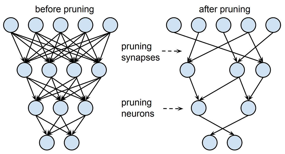
• Quantization-aware training can be more complex to implement. PruningThis involves removing redundant or less important connections (weights) in a neural network. The idea is that many large models have a significant number of parameters that contribute very little to the model's overall performance. By removing these parameters, we can reduce the model size and computational cost.

How it works:

Pruning techniques typically involve:

• Identifying unimportant weights: Various criteria can be used to determine the importance of a weight, such as its magnitude (smaller magnitudes are often considered less important), its contribution to the loss, or gradient-based methods.
• Removing (setting to zero) the unimportant weights: Once identified, these weights are set to zero, effectively removing the corresponding connections in the network.
• Fine-tuning (optional but often necessary): After pruning, the remaining weights are often fine-tuned on the training data to recover any potential loss in accuracy due to the removal of weights.
• Sparse representation: To realize the benefits of reduced computation, the pruned model (with many zero weights) often needs to be stored and processed using sparse matrix representations, which can skip the zero-valued operations. Specialized hardware or software libraries are often required to efficiently exploit this sparsity.When to use:

Pruning is useful when you have a large, over-parameterized model and want to reduce its size and inference time without significant accuracy degradation. It can be applied to various types of neural networks.

Benefits:

• Reduction in model size: Removing a significant portion of the weights can lead to substantial size reduction.

• Faster inference speed: Fewer computations are required during inference if the sparsity can be efficiently exploited.

• Lower power consumption: Reduced computations can lead to lower energy usage.Risks:

• Potential loss of accuracy: Aggressive pruning can lead to a significant drop in performance.

• Requires specialized hardware or software for efficient inference: Simply having many zero weights doesn't automatically lead to faster computation. Sparse matrix operations need to be efficiently supported.

• Can make the model architecture irregular: The resulting sparse structure can be challenging to implement efficiently on standard hardware.

• The pruning process itself can be computationally expensive and require careful hyperparameter tuning (e.g., the pruning rate and schedule). Knowledge DistillationKnowledge distillation is a technique where a smaller "student" model is trained to mimic the behavior of a larger, more complex, and often more accurate "teacher" model. The teacher model transfers its "knowledge" to the student, enabling the student to achieve better performance than it would if trained solely on the original training data.How it works:

The teacher model, which has already been trained to high accuracy, is used to generate "soft targets" for the training data.

Soft targets are the probability distributions over the classes produced by the teacher's output layer. These soft targets contain more information about the relationships between classes than the hard labels (the ground truth one-hot encoded vectors).

The student model is then trained to not only match the hard labels but also to reproduce these soft targets from the teacher. This additional learning signal from the teacher helps the student learn more nuanced representations and generalize better.

When to use it:

** **Knowledge distillation is useful when you have a very accurate but computationally expensive teacher model and you want to create a smaller, faster student model for deployment, especially in resource-constrained environments.

It can also be used to transfer knowledge from ensemble models to a single, more manageable model.

Benefits:

• Smaller student model: The student model can be significantly smaller and faster than the teacher.

• Improved performance of the student model: By learning from the teacher's soft targets, the student can often achieve higher accuracy than if trained independently with the same architecture and data.

• Can transfer knowledge from complex models or ensembles: Distillation allows you to distill the knowledge captured in large or multiple models into a single, efficient model.Risks:

• Requires a pre-trained teacher model: The effectiveness of knowledge distillation relies on having a well-performing teacher model.

• The design of the student model is still important: The student model needs to have sufficient capacity to learn the knowledge from the teacher.

• The distillation process introduces new hyperparameters (e.g., the temperature parameter used to soften the teacher's probabilities) that need to be tuned.

• The student's performance is upper-bounded by the teacher's performance.

These model compression techniques, often used in combination, play an important role in making advanced ML models more practical and deployable in a wider range of applications.

The choice of which technique to use depends on the specific requirements of the deployment environment, the acceptable trade-off between model size/speed and accuracy, and the characteristics of the model and the data.

Key points

In this session, we explored how adaptive learning rate methods like Adam, RMSprop, and Adagrad can improve model training by automatically adjusting learning rates for better performance and faster convergence.

We also looked at model compression techniques such as quantization, pruning, and knowledge distillation, which help reduce model size and computational cost without sacrificing accuracy.

By applying these methods, you can build models that not only perform well but are also optimized for deployment across a variety of platforms and environments.

Knowledge check

Before moving on, see if you can apply what you've learned by answering the knowledge check questions below.

Ensemble methods

What’s smarter than a ML model? A team of them.

Individually, models can be fragile and inconsistent—but combine them, and you unlock the power of collective intelligence. Just like a panel of experts reaches better conclusions than a single voice, ensemble methods blend the strengths of multiple models to deliver more accurate, reliable, and robust predictions.

Ready to find out how this works in practice?

Ensemble methods

Sometimes, an individual ML model might not be very powerful on its own. For example, decision trees can produce different results each time they are run on the same data depending on which path the algorithm follows.

An ensemble method is when we combine the predictions of several “base” or “weak” learners to make a final prediction. The idea is that a group of diverse models together can achieve better predictive accuracy and generalization than on their own.

You can think of it like “crowd-sourcing” a prediction, where each model provides its output and the one which is most common is selected.

Ensemble methods help us:

• Reduce both bias and variance through aggregating the outputs of multiple models, leading to more accurate predictions.
• Enhance model robustness and stability by overcoming errors in individual models i.e. if one model makes an error, the others might still predict correctly.
• Get better generalization to unseen data by combining diverse perspectives, reducing the risk of overfitting. Let’s take a look at a couple of methods.

**Bagging (Bootstrap Aggregating)**This is a parallel ensemble method that aims to reduce the variance of a base learner. It involves training multiple instances of the same model (the base learners) on different subsets of the training data.

These subsets are created randomly by sampling the original data with replacement (called bootstrapping). Once each model has been trained, their predictions are aggregated to produce the final prediction.

Random Forest is a popular bagging algorithm that uses decision trees as base learners.

How it works:

• For each base learner B, we create a bootstrap sample of size N from the training data with replacement (this means that some data points might be included multiple times in a single bootstrap sample).
• Each base learner (e.g. decision tree or neural network) is trained independently on its bootstrap sample.
• When we want to make a prediction, we do so with each base learner and aggregate the results.Classification: Each base learner makes a class prediction, with the final prediction being the class that receives the majority of the “votes”.
• Regression: Each base learner predicts a numerical value which is averaged.

When to use it:

• When the base learner is prone to high variance (overfitting). Decision trees (especially deep learning ones) tend to be sensitive to specific training data, so bagging is a common choice.

• When we want to improve the stability and accuracy of a single model. Benefits:

• Reduced variance: By training on different bootstrap samples and aggregating the results, bagging smooths out the predictions and reduces the impact of high-variance base learners.

• Improved stability: The ensemble is less likely to be drastically affected by small changes in the training data.

• Relatively easy to implement: The process of bootstrap sampling and independent training of base learners is conceptually straightforward.

• Out-of-Bag (OOB) error estimation: Since each base learner is trained on a subset of the data, the data points not included in that specific bootstrap sample (on average, about 37% of the data) can be used as a validation set to estimate the model's performance without the need for a separate validation set. This is known as the OOB error.Risks:

• Increased bias (potentially): While primarily aimed at reducing variance, if the base learners are already highly biased, bagging might not significantly reduce this bias and could even slightly increase it in some cases.

• Reduced interpretability: Ensembles are generally less interpretable than single models, as you are dealing with the combined predictions of multiple learners.

• Computational cost: Training multiple base learners can be computationally expensive, especially if the base learners themselves are complex or the number of learners in the ensemble is large.BoostingThis is a sequential ensemble method that aims to reduce the bias and variance of a base learner.

Unlike bagging, where base learners are trained independently, in boosting, each new base learner is trained to focus on the mistakes made by the previous learners. The learners are combined using a weighted sum (for regression) or a weighted majority vote (for classification), where more weight is given to the better-performing learners

AdaBoost, Gradient Boosting (GBM), XGBoost, LightGBM and CatBoost are popular boosting algorithms.

How it works:

• The base learners are trained sequentially.
• Each data point in the training set is assigned a weight (initially all weights are equal).
• In each iteration, the new base learner is trained on the re-weighted data, with higher weights given to the data points that were misclassified (or had larger errors) by the previous learners. This forces the new learner to focus on the difficult instances.
• Each trained base learner is assigned a weight based on its performance. More accurate learners typically receive higher weights in the final aggregation.
• Finally, the predictions from the base learners are aggregated.Classification: Each base learner makes a prediction. The final prediction is determined by a weighted majority vote (i.e. more accurate learners get more votes).
• Regression: Each base learner predicts a value. The final prediction is a weighted average.

When to use it:

• When we want to reduce both bias and variance and achieve higher accuracy than a single model can provide.

• When the base learner is relatively weak (slightly better than random guessing). Simple models like shallow decision trees (stumps) are often used as base learners in boosting. Benefits:

• High accuracy: Boosting algorithms often achieve very high predictive accuracy by iteratively improving the model's performance on difficult instances.

• Bias reduction: By focusing on the errors of previous learners, boosting can effectively reduce the bias of the overall ensemble.

• Feature importance: Some boosting algorithms (like Gradient Boosting and XGBoost) provide a measure of feature importance, which can be useful for understanding the data and the model's decision-making process.Risks:

• Sensitivity to noisy data and outliers: Boosting algorithms can be sensitive to noisy data and outliers, as they try to correct every single misclassification, which might lead to overfitting the noise.

• Potential for overfitting: If the boosting process continues for too many iterations, the model can start to overfit the training data. Careful tuning of hyperparameters (e.g., the number of boosting rounds, learning rate) and the use of regularization techniques are crucial.

• Computational cost: Sequential training can be computationally expensive, especially if the base learners are complex or the number of boosting rounds is large.

• Interpretability: Similar to bagging, boosted ensembles are generally less interpretable than single models.StackingFinally stacking (or stacked generalization) is a method that combines the prediction of multiple different base learners by training a new model called a “meta-learner” or “aggregator” to learn how to best combine the base learner’s predictions.

Unlike bagging or boosting, the base learners in stacking are typically different types of model. For example, you might use a Random Forest, Gradient Boosting machine and a Support Vector Machine as the base learners, with a Logistic Regression as the meta-learner.

The predictions of the three base learners on the validation set (or using cross-validation) would be used as features to train the Logistic Regression model to make the final prediction.

How it works:

• Several different base learners (e.g. Random Forest, SVM and Gradient Boosting) are trained on the original training data (called Level-0 models).
• The trained base learners are then used to make predictions on the original training data. Often out-of-fold predictions from a cross-validation procedure are used to avoid information leakage. These predictions become the “meta-features” or “Level-1” data.
• A meta-learner (e.g. Logistic Regression) is trained on these meta-features, with the original target variable as the output. The meta-learner learns how to weigh the predictions of the base learners to make the final prediction.
• For a new, unseen data point, the base learners first make their predictions. These predictions are then fed as input to the trained meta-learners, which outputs the final ensemble prediction.

When to use it:

• When we have a diverse set of well-performing base learners and we believe that a meta-learner can learn to effectively combine their strengths.

• When the base learners make different types of errors, and we want a model that can learn to correct these errors based on the other learners' predictions. Benefits:

• Potential for high accuracy: Stacking can often achieve higher accuracy than individual base learners by optimally combining their predictions.

• Combine the strengths of different models: It allows you to combine models that excel in different aspects of the data or make different types of predictions.

• Flexibility: You can choose different types of base learners and a suitable meta-learner for your specific problem.Risks:

• Increased complexity: Stacking introduces more complexity to the modeling process, with the need to train multiple base learners and a meta-learner.

• Risk of overfitting: If the meta-learner is too complex or the process is not carefully implemented (e.g., without using cross-validation to generate meta-features), there is a risk of overfitting the meta-learner to the predictions of the base learners on the training data.

• Reduced interpretability: Stacked ensembles are generally even less interpretable than bagged or boosted ensembles due to the multiple layers of models involved.

• Computational cost: Training multiple diverse base learners and a meta-learner can be computationally expensive.

If you are using models which can risk having high variance or bias, ensemble methods have the potential to help you overcome these issues. Why not try researching one of these model types and running them with your analysis.

Key points

Ensemble methods help overcome the limitations of individual models by combining their predictions to improve accuracy, stability, and generalization.

Whether using bagging to reduce variance, boosting to reduce bias, or stacking to combine the strengths of different model types, these approaches allow you to build more powerful solutions.

By applying ensemble techniques in your role, you can create models that better handle complex datasets, mitigate errors, and provide more dependable insights for decision-making.

Knowledge check

Before moving on, see if you can apply what you've learned by answering the knowledge check questions below.